Signal Processing - Nyquist Sampling Theorem

Nyquist Sampling Theorem

A continuous time signal can be represented in its samples and can be recovered back when sampling frequency f_s is greater than or equal to the twice the highest frequency component of message signal.

fs≥2fm

The Nyquist Theorem, also known as the sampling theorem, is a principle that engineers follow in the digitization of analog signals. For analog-to-digital conversion (ADC) slices, called samples, of the analog waveform must be taken frequently. The number of samples per second is called the sampling rate or sampling frequency.

As tube amplifiers give a more pleasant mutation and compression to musical signals than transistors, analog tape similarly warms up and fattens the sound. Though, it is not needed to refrain from the other different uses of it. Other techniques such as tube compressors, to fatten the sound if needed. 

there is no such thing as the perfect low-pass filter required by Nyquist’s theorem. A real filter has a finite slope, so the cut-off should be kept a little lower than theory. Also, a steep filter has a lot of phase shift near and above the cutoff. And some aliasing is bound to leak through at the very high end. A technique called over sampling has been developed to reduce these problems.

Another huge problem is finite word length effects- using 16-bit samples, not the pure numbers of the Nyquist theorem, so standards to the sample values. as for the start 16 bits is not a big deal, but as it transforms into 96 dynamic range it comes to an extent which it cannot be exceeded further more.  So, the average music level must be much lower in order to allow headroom for peaks. And, at the low amplitude end, distortion of small-signal components is very high. On top of this, any gain change (from mixing tracks or changing volumes) causes individual samples to be rounded to the nearest bit level, adding distortion. To overcome that, a technique called dithering relieves these problems.

Proof of Nyquist Shanon Sampling Theorem

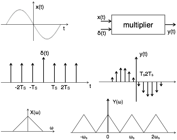
Here, you can observe that the sampled signal takes the period of impulse. The process of sampling can be explained by the following mathematical expression:

Sampled signaly(t)=x(t).δ(t)......(1)$\text{Sampled signal}y(t)=x(t).\delta (t)......(1)$

The trigonometric Fourier series representation of δ$\delta$(t) is given by

δ(t)=a0+Σ∞n=1(ancosnωst+bnsinnωst)......(2)$\delta (t)=a_0+{\mathrm{\Sigma }}_{n=1}^{\mathrm{\infty }}(a_n\cos n{\omega }_{s}t+b_n\sin n{\omega }_{s}t)......(2)$

Where a0=1Ts∫T2−T2δ(t)dt=1Tsδ(0)=1Ts$a_0=\frac{1}{T_s}{\int }_{\frac{-T}{2}}^{\frac{T}{2}}\delta (t)dt=\frac{1}{T_s}\delta (0)=\frac{1}{T_s}$

an=2Ts∫T2−T2δ(t)cosnωsdt=2T2δ(0)cosnωs0=2T$a_n=\frac{2}{T_s}{\int }_{\frac{-T}{2}}^{\frac{T}{2}}\delta (t)\cos n{\omega }_{s}dt=\frac{2}{T_2}\delta (0)\cos n{\omega }_{s}0=\frac{2}{T}$

bn=2Ts∫T2−T2δ(t)sinnωstdt=2Tsδ(0)sinnωs0=0$b_n=\frac{2}{T_s}{\int }_{\frac{-T}{2}}^{\frac{T}{2}}\delta (t)\sin n{\omega }_{s}tdt=\frac{2}{T_s}\delta (0)\sin n{\omega }_{s}0=0$

Substitute above values in equation 2.

∴δ(t)=1Ts+Σ∞n=1(2Tscosnωst+0)$\therefore \delta (t)=\frac{1}{T_s}+{\mathrm{\Sigma }}_{n=1}^{\mathrm{\infty }}(\frac{2}{T_s}\cos n{\omega }_{s}t+0)$

Substitute δ(t) in equation 1.

→y(t)=x(t).δ(t)$\to y(t)=x(t).\delta (t)$

=x(t)[1Ts+Σ∞n=1(2Tscosnωst)]$=x(t)[\frac{1}{T_s}+{\mathrm{\Sigma }}_{n=1}^{\mathrm{\infty }}(\frac{2}{T_s}\cos n{\omega }_{s}t)]$

=1Ts[x(t)+2Σ∞n=1(cosnωst)x(t)]$=\frac{1}{T_s}[x(t)+2{\mathrm{\Sigma }}_{n=1}^{\mathrm{\infty }}(\cos n{\omega }_{s}t)x(t)]$

y(t)=1Ts[x(t)+2cosωst.x(t)+2cos2ωst.x(t)+2cos3ωst.x(t)......]$y(t)=\frac{1}{T_s}[x(t)+2\cos {\omega }_{s}t.x(t)+2\cos 2{\omega }_{s}t.x(t)+2\cos 3{\omega }_{s}t.x(t)......]$

Take Fourier transform on both sides.

Y(ω)=1Ts[X(ω)+X(ω−ωs)+X(ω+ωs)+X(ω−2ωs)+X(ω+2ωs)+...]$Y(\omega )=\frac{1}{T_s}[X(\omega )+X(\omega -{\omega }_s)+X(\omega +{\omega }_s)+X(\omega -2{\omega }_s)+X(\omega +2{\omega }_s)+...]$

∴Y(ω)=1TsΣ∞n=−∞X(ω−nωs)wheren=0,±1,±2,...$\therefore Y(\omega )=\frac{1}{T_s}{\mathrm{\Sigma }}_{n=-\mathrm{\infty }}^{\mathrm{\infty }}X(\omega -n{\omega }_s)wheren=0,\pm 1,\pm 2,...$

To reconstruct x(t), you must recover input signal spectrum X(ω) from sampled signal spectrum Y(ω), which is possible when there is no overlapping between the cycles of Y(ω).

Possibility of sampled frequency spectrum with different conditions is given by the following diagrams:

Reference 1 

Reference 2

Author : Pavarindu Sahansith